Drawing vector field
by tsulej
folds2d.tumblr.com

The goal
During last few days I’ve made several attempts to create and visualize 2D vector fields. In the following article you can read about this concept with several examples and code in Processing.
There are many beautiful art/code based on vector field visualization around the net. Mostly based on noise function. Check them out before you start:
- Visualizer by p5art
- Furfrolic by Holger Lippmann
- My own two sketches drawing_generative and threadraw
- Few examples on OpenProcessing site: 1, 2, 3, 4
What is the vector field?
Vector field (in our case) is just a 
Why vector? Because you can treat a pair of 

Vector fields can be visualised in the following way


How to get the vector field
The main goal, in this article, is to research various ways to create vector fields. There two cases.
We can operate on functions which returns pair of values like variations. In this case such function defines vector field itself. We can use also some vector operations (like substraction, sum, etc…) to get new functions.
The second option is to get single float number 
Drawing method
The method is quite simple.
- Create points from
floating point range
- Draw them
- For each of the point calculate relating vector from the vector field
- Scale it and add to the point coordinates
- Repeat 2-4
Step 4 is key here. We move our points along vectors. Trace lines build the resulting image.
The general flow for constructing vector field follows this scheme:
![p=(x,y)\mapsto [multiple operations]\mapsto \vec{v}](https://s0.wp.com/latex.php?latex=p%3D%28x%2Cy%29%5Cmapsto+%5Bmultiple+operations%5D%5Cmapsto+%5Cvec%7Bv%7D&bg=fff&fg=444444&s=0&c=20201002)
Note: I assume that on every step I can multiply function variables or returned values by any number.
Here is code stub for my experiments
// dynamic list with our points, PVector holds position
ArrayList<PVector> points = new ArrayList<PVector>();

// colors used for points
color[] pal = {
  color(0, 91, 197),
  color(0, 180, 252),
  color(23, 249, 255),
  color(223, 147, 0),
  color(248, 190, 0)
};

// global configuration
float vector_scale = 0.01; // vector scaling factor, we want small steps
float time = 0; // time passes by

void setup() {
  size(800, 800);
  strokeWeight(0.66);
  background(0, 5, 25);
  noFill();
  smooth(8);

  // noiseSeed(1111); // sometimes we select one noise field

  // create points from [-3,3] range
  for (float x=-3; x<=3; x+=0.07) {
    for (float y=-3; y<=3; y+=0.07) {
      // create point slightly distorted
      PVector v = new PVector(x+randomGaussian()*0.003, y+randomGaussian()*0.003);
      points.add(v);
    }
  }
}

void draw() {
  int point_idx = 0; // point index
  for (PVector p : points) {
    // map floating point coordinates to screen coordinates
    float xx = map(p.x, -6.5, 6.5, 0, width);
    float yy = map(p.y, -6.5, 6.5, 0, height);

    // select color from palette (index based on noise)
    int cn = (int)(100*pal.length*noise(point_idx))%pal.length;
    stroke(pal[cn], 15);
    point(xx, yy); //draw

    // placeholder for vector field calculations

    // v is vector from the field
    PVector v = new PVector(0, 0);

    p.x += vector_scale * v.x;
    p.y += vector_scale * v.y;

    // go to the next point
    point_idx++;
  }
  time += 0.001;
}
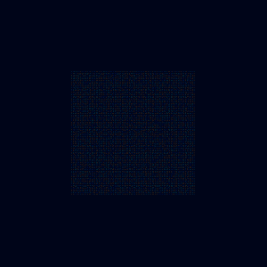
When I change my field vector to be constant one (different than 0), my points start move.
PVector v = new PVector(0.1, 0.1);

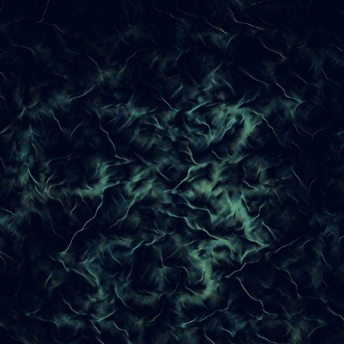
Perlin noise
Let’s begin with perlin noise in few configurations. I’m going to change only marked lines from the code stub.
Variant 1
noise(x,y) function in processing returns value from 0 to 1 (actually implementation used in Processing has some problems and real value is often in range from 0.2 to 0.8). I will treat resulted value as an angle in polar coordinates and use sin()/cos() functions to convert it to cartesian ones. To properly do this I have to scale it up to range ![[0,2\pi ]](https://s0.wp.com/latex.php?latex=%5B0%2C2%5Cpi+%5D&bg=fff&fg=444444&s=0&c=20201002)
![[-\pi, \pi ]](https://s0.wp.com/latex.php?latex=%5B-%5Cpi%2C+%5Cpi+%5D&bg=fff&fg=444444&s=0&c=20201002)
// placeholder for vector field calculations
float n = TWO_PI * noise(p.x,p.y);
PVector v = new PVector(cos(n),sin(n));

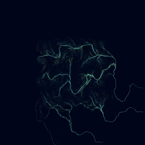
Variant 2
Let’s check what happens when I multiply noise by 10, 100, 300 or even 1000. Noise is now scaled to range ![[-1.1]](https://s0.wp.com/latex.php?latex=%5B-1.1%5D&bg=fff&fg=444444&s=0&c=20201002)
float n = 10 * map(noise(p.x/5,p.y/5),0,1,-1,1); // 100, 300 or 1000
PVector v = new PVector(cos(n),sin(n));


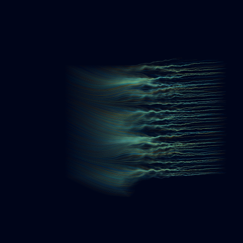
Variant 3
Two of above variants were using classic method. Now I get rid of polar->cartesian conversion and I’m going to treat returned value from noise() as cartesian coordinates. Angle of the vector is the same for whole field and only length of vector is changed. This leads to some interesting patterns. Experiment with scaling input coordinates and
float n = 5*map(noise(p.x,p.y),0,1,-1,1);
PVector v = new PVector(n,n);


Parametric curves
Let’s use parametric curves to convert noise() result into vector. The big list of them is defined in Wolfram Alpha or named here. Parametric curve (or plane curve) is a function 
Astroid
// placeholder for vector field calculations
float n = 5*map(noise(p.x,p.y),0,1,-1,1); // and 2

float sinn = sin(n);
float cosn = cos(n);

float xt = sq(sinn)*sinn;
float yt = sq(cosn)*cosn;

PVector v = new PVector(xt,yt);
Results for noise scale 2 and 5


Cissoid of Diocles
// placeholder for vector field calculations
float n = 3*map(noise(p.x,p.y),0,1,-1,1);

float sinn2 = 2*sq(sin(n));

float xt = sinn2;
float yt = sinn2*tan(n);

PVector v = new PVector(xt,yt);

Kampyle of Eudoxus
// placeholder for vector field calculations
float n = 6*map(noise(p.x,p.y),0,1,-1,1);

float sec = 1/sin(n);

float xt = sec;
float yt = tan(n)*sec;

PVector v = new PVector(xt,yt);
Rectangular Hyperbola
// placeholder for vector field calculations
float n = 10*map(noise(p.x*2,p.y*2),0,1,-1,1);

float xt = 1/sin(n);
float yt = tan(n);

PVector v = new PVector(xt,yt);

Superformula
// placeholder for vector field calculations
float n = 5*map(noise(p.x,p.y),0,1,-1,1);

float a = 1;
float b = 1;
float m = 6;
float n1 = 1;
float n2 = 7;
float n3 = 8;

float f1 = pow(abs(cos(m*n/4)/a),n2);
float f2 = pow(abs(sin(m*n/4)/b),n3);
float fr = pow(f1+f2,-1/n1);

float xt = cos(n)*fr;
float yt = sin(n)*fr;

PVector v = new PVector(xt,yt);
Noise and curves combined
Now I’m going to play with some combinations of above curves and make multiple passes through noise().
Let’s put all curves into functions (paste following code to the end of the script):
PVector circle(float n) { // polar to cartesian coordinates
  return new PVector(cos(n), sin(n));
}

PVector astroid(float n) {
  float sinn = sin(n);
  float cosn = cos(n);

  float xt = sq(sinn)*sinn;
  float yt = sq(cosn)*cosn;

  return new PVector(xt, yt);
}

PVector cissoid(float n) {
  float sinn2 = 2*sq(sin(n));

  float xt = sinn2;
  float yt = sinn2*tan(n);

  return new PVector(xt, yt);
}

PVector kampyle(float n) {
  float sec = 1/sin(n);

  float xt = sec;
  float yt = tan(n)*sec;

  return new PVector(xt, yt);
}

PVector rect_hyperbola(float n) {
  float sec = 1/sin(n);

  float xt = 1/sin(n);
  float yt = tan(n);

  return new PVector(xt, yt);
}

final static float superformula_a = 1;
final static float superformula_b = 1;
final static float superformula_m = 6;
final static float superformula_n1 = 1;
final static float superformula_n2 = 7;
final static float superformula_n3 = 8;
PVector superformula(float n) {
  float f1 = pow(abs(cos(superformula_m*n/4)/superformula_a), superformula_n2);
  float f2 = pow(abs(sin(superformula_m*n/4)/superformula_b), superformula_n3);
  float fr = pow(f1+f2, -1/superformula_n1);

  float xt = cos(n)*fr;
  float yt = sin(n)*fr;

  return new PVector(xt, yt);
}
Variant 1 – p5art
Code based on p5art web app noisePainting

// placeholder for vector field calculations
float n1 = 10*noise(1+p.x/20, 1+p.y/20); // shift input to avoid symetry
float n2 = 5*noise(n1, n1);
float n3 = 325*map(noise(n2, n2), 0, 1, -1, 1); // 25,325

PVector v = circle(n3);


Variant 2

// placeholder for vector field calculations
float n1 = 15*map(noise(1+p.x/20, 1+p.y/20),0,1,-1,1);

PVector v1 = cissoid(n1);
PVector v2 = astroid(n1);

float n2a = 5*noise(v1.x,v2.y);
float n2b = 5*noise(v2.x,v1.y);

float n3 = 10*map(noise(n2a, n2b/3), 0, 1, -1, 1);

PVector v = circle(n3);

Variant 3

// placeholder for vector field calculations
float n1 = 15*map(noise(1+p.x/10, 1+p.y/10),0,1,-1,1);

PVector v1 = rect_hyperbola(n1);
PVector v2 = astroid(n1);

float n2a = 2*map(noise(v1.x,v1.y),0,1,-1,1);
float n2b = 2*map(noise(v2.x,v2.y),0,1,-1,1);

PVector v = new PVector(n2a,n2b);

Variant 4

// placeholder for vector field calculations
PVector v1 = kampyle(p.x);
PVector v2 = superformula(p.y);

float n2a = 3*map(noise(v1.x,v1.y),0,1,-1,1);
float n2b = 3*map(noise(v2.x,v2.y),0,1,-1,1);

PVector v = new PVector(cos(n2a),sin(n2b));

Variant 5

// placeholder for vector field calculations
float n1a = 3*map(noise(p.x,p.y),0,1,-1,1);
float n1b = 3*map(noise(p.y,p.x),0,1,-1,1);

PVector v1 = rect_hyperbola(n1a);
PVector v2 = astroid(n1b);

float n2a = 3*map(noise(v1.x,v1.y),0,1,-1,1);
float n2b = 3*map(noise(v2.x,v2.y),0,1,-1,1);

PVector v = new PVector(cos(n2a),sin(n2b));

Variant 6 – comparison
Here I want to compare different curves using the same method. I change marked lines into pair of curves defined above. I’ve put noiseSeed(1111); in setup() to have the same noise structure. Check image description to see what curves were used.

// placeholder for vector field calculations
float n1a = 15*map(noise(p.x/10,p.y/10),0,1,-1,1);
float n1b = 15*map(noise(p.y/10,p.x/10),0,1,-1,1);

PVector v1 = superformula(n1a);
PVector v2 = circle(n1b);

PVector diff = PVector.sub(v2,v1);
diff.mult(0.3);

PVector v = new PVector(diff.x,diff.y);


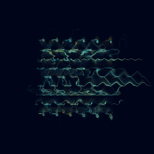
Time
Now let’s introduce time. An external variable which is incremented every frame with some small value. It can be used to slightly change noise field during rendrering or can be used as a scale factor.
Let’s compare the same vector field without time and time used as third noise parameter.
 // placeholder for vector field calculations
 float n1a = 3*map(noise(p.x/2,p.y/2),0,1,-1,1);
 float n1b = 3*map(noise(p.y/2,p.x/2),0,1,-1,1);
 float nn = 6*map(noise(n1a,n1b),0,1,-1,1);

 PVector v = circle(nn);

And now I add time as a third parameter to noise function. This way our vector field changes when time passes.
 // placeholder for vector field calculations
float n1a = 3*map(noise(p.x/2,p.y/2,time),0,1,-1,1);
float n1b = 3*map(noise(p.y/2,p.x/2,time),0,1,-1,1);
float nn = 6*map(noise(n1a,n1b,time),0,1,-1,1);

PVector v = circle(nn);

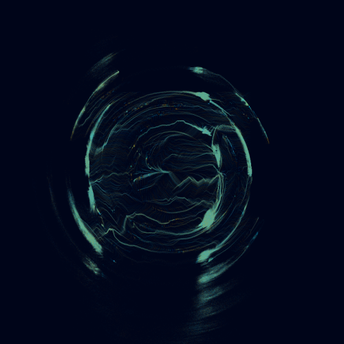
Now time is used as a scaling factor.
// placeholder for vector field calculations
float n1a = 3*map(noise(p.x/2,p.y/2),0,1,-1,1);
float n1b = 3*map(noise(p.y/2,p.x/2),0,1,-1,1);

float nn = time*10*6*map(noise(n1a,n1b),0,1,-1,1);

PVector v = circle(nn);

Variations
Now let’s introduce variations (see previous post about Folds) as a vector field definition.
Copy below code to the end of your sketch. It includes function definiotions used in this and next chapters.
PVector sinusoidal(PVector v, float amount) {
  return new PVector(amount * sin(v.x), amount * sin(v.y));
}

PVector waves2(PVector p, float weight) {
  float x = weight * (p.x + 0.9 * sin(p.y * 4));
  float y = weight * (p.y + 0.5 * sin(p.x * 5.555));
  return new PVector(x, y);
}

PVector polar(PVector p, float weight) {
  float r = p.mag();
  float theta = atan2(p.x, p.y);
  float x = theta / PI;
  float y = r - 2.0;
  return new PVector(weight * x, weight * y);
}

PVector swirl(PVector p, float weight) {
  float r2 = sq(p.x)+sq(p.y);
  float sinr = sin(r2);
  float cosr = cos(r2);
  float newX = 0.8 * (sinr * p.x - cosr * p.y);
  float newY = 0.8 * (cosr * p.y + sinr * p.y);
  return new PVector(weight * newX, weight * newY);
}

PVector hyperbolic(PVector v, float amount) {
  float r = v.mag() + 1.0e-10;
  float theta = atan2(v.x, v.y);
  float x = amount * sin(theta) / r;
  float y = amount * cos(theta) * r;
  return new PVector(x, y);
}

PVector power(PVector p, float weight) {
  float theta = atan2(p.y, p.x);
  float sinr = sin(theta);
  float cosr = cos(theta);
  float pow = weight * pow(p.mag(), sinr);
  return new PVector(pow * cosr, pow * sinr);
}

PVector cosine(PVector p, float weight) {
  float pix = p.x * PI;
  float x = weight * 0.8 * cos(pix) * cosh(p.y);
  float y = -weight * 0.8 * sin(pix) * sinh(p.y);
  return new PVector(x, y);
}

PVector cross(PVector p, float weight) {
  float r = sqrt(1.0 / (sq(sq(p.x)-sq(p.y)))+1.0e-10);
  return new PVector(weight * 0.8 * p.x * r, weight * 0.8 * p.y * r);
}

PVector vexp(PVector p, float weight) {
  float r = weight * exp(p.x);
  return new PVector(r * cos(p.y), r * sin(p.y));
}

// parametrization P={pdj_a,pdj_b,pdj_c,pdj_d}
float pdj_a = 0.1;
float pdj_b = 1.9;
float pdj_c = -0.8;
float pdj_d = -1.2;
PVector pdj(PVector v, float amount) {
  return new PVector( amount * (sin(pdj_a * v.y) - cos(pdj_b * v.x)),
  amount * (sin(pdj_c * v.x) - cos(pdj_d * v.y)));
}

final float cosh(float x) { return 0.5 * (exp(x) + exp(-x));}
final float sinh(float x) { return 0.5 * (exp(x) - exp(-x));}
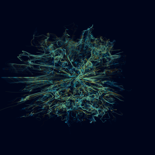
Let’s see how individual variations look as vector fields. Sometimes I had to adjust scaling factor to keep points on the screen.
// placeholder for vector field calculations
PVector v = sinusoidal(p,1);
v.mult(1); // different values for different functions


All together
Let’s sumarize what functions we have now defined.
- multiplying/dividing by number
- single variable noise()
- other single variable functions (sin/cos, exp, log, sq, sqrt, etc.)
- parametric curves
- noise() with two parameters
- distance between vectors
- dot product of vectors
- length of the vector
- angle between vectors
- variations and their combinations
- sum or difference of vectors
- atan2() of the vector


All above operations can be used to generate vector field (or simply transform 2d point to another 2d point).
I will play with above transformations in following examples. It’s a record of experiments.
Variant 1

// placeholder for vector field calculations
float n1 = 5*map(noise(p.x/5,p.y/5),0,1,-1,1);

PVector v1 = rect_hyperbola(n1);
PVector v2 = swirl(v1,1);

PVector v = new PVector(cos(v2.x),sin(v2.y));

Variant 2

// placeholder for vector field calculations
float n1 = 5*map(noise(p.x/5,p.y/5),0,1,-1,1);
float n2 = 5*map(noise(p.y/5,p.x/5),0,1,-1,1);

PVector v1 = vexp(new PVector(n1,n2),1);
PVector v2 = swirl(new PVector(n2,n1),1);

PVector v3 = PVector.sub(v2,v1);

PVector v4 = waves2(v1,1);
v4.mult(0.8);

PVector v = new PVector(v4.x,v4.y);

Variant 3

// placeholder for vector field calculations
PVector v1 = vexp(p,1);

float n1 = map(noise(v1.x,v1.y,time),0,1,-1,1);
float n2 = map(noise(v1.y,v1.x,-time),0,1,-1,1);

PVector v2 = vexp(new PVector(n1,n2),1);

PVector v = new PVector(v2.x,v2.y);
Variant 4

// placeholder for vector field calculations
PVector v1 = polar(cross(p,1),1);

float n1 = 15*map(noise(v1.x,v1.y,time),0,1,-1,1);
PVector v2 = cissoid(n1);
v2.normalize();

PVector v = new PVector(v2.x,v2.y);

Variant 5

// placeholder for vector field calculations
PVector v1 = power(p,1);

float n1 = 5*map(noise(v1.x,v1.y,time),0,1,-1,1);
float n2 = 5*map(noise(p.x/3,p.y/3,-time),0,1,-1,1);

PVector v2 = cosine(new PVector(n1,n2),1);

float a1 = PVector.angleBetween(v1,v2);

PVector v3 = superformula(a1);
v3.mult(3);

PVector v = new PVector(cos(v3.x),sin(v3.y));
Variant 6

// placeholder for vector field calculations
PVector v1 = waves2(p,1);
PVector v2 = PVector.sub(v1,p);

float n1 = 8*noise(time)*atan2(v1.y,v1.x);
float n2 = 8*noise(time+0.5)*atan2(v2.y,v2.x);

PVector v = new PVector(cos(v2.x*n1),sin(v1.y+n2));
Variant 7

// placeholder for vector field calculations
PVector v1 = swirl(p,1);
v1.mult(0.5);
PVector v2 = PVector.sub(v1,p);

float nv1 = noise(v1.x,v1.y,time);
float nv2 = noise(v2.x,v2.y,-time);

float n1 = (atan2(v1.y,v1.x)+nv2);
float n2 = (atan2(v2.y,v2.x)+nv1);

PVector v3 = superformula(n1);
PVector v4 = rect_hyperbola(n2);

PVector tv3 = waves2(v3,1);
PVector tv4 = sinusoidal(v4,1);

PVector v5 = PVector.sub(tv4,tv3);

PVector v6 = pdj(v5,1);

float an = PVector.angleBetween(v6,new PVector(n1,n2));

PVector v = new PVector(cos(v2.x+sin(an)),sin(v6.y-cos(an)));
v.mult(1+time*40);
Image
The last part is about using channel information from an image as a vector field. I wrote two sketches some time ago which are based on vector field concept.
Drawing generative

Threadraw

How to use image data
First load your image at the beginning of the sketch
img = loadImage("natalie.jpg"); // PImage img; must be declared globally
Then use image data following way
// placeholder for vector field calculations
PVector v1 = sinusoidal(p,1);

int img_x = (int)map(p.x,-3,3,0,img.width);
int img_y = (int)map(p.y,-3,3,0,img.height);

float b = brightness( img.get(img_x,img_y) )/255.0;
PVector br = circle(b);

float a = 5*PVector.angleBetween(br,v1);

PVector v = astroid(a);

Appendix
This concept is taken from zach lieberman and Keith Peters who explored painting by non-intersecting segments. This idea can be used on vector fields too. Here are two examples.


See the code HERE.
The end
Questions? generateme.blog@gmail.com or Follow @generateme_blog

I’m wondering if I can mask a set of points to make a certain shape (A circle, for example) from an image.
Btw very nice tutorial!
LikeLiked by 1 person
Thx! I’m not sure if I understand properly. Could you elaborate a little bit more?
LikeLike
Hello, I’m interested in all this now.
I find it fascinating!
I do not understand which program you use, how do you do this …. etc …. it would be nice to fix this somewhere on the site, such as “first steps” …
Would you help me?
LikeLike
Hi, all is done in Processing.
https://processing.org/ All necessary tutorials how to start are there.
LikeLiked by 1 person
Thank you! Very simplified! keep doing this great job 🙂
LikeLike
I’m testing and I would like the particles to live longer … the lines would be longer …
They’re running out too soon.
Is it possible to change it?
LikeLike
There is no limit for particle life time. Particles can be stacked when field velocity is near zero.
LikeLiked by 1 person
Was it probably this way that this artist achieved these results?
https://www.tfmstyle.com/retina-pack/
Wonderful
LikeLike
Definitely these are achived by using particle system. I don’t know what formula is behind. I’ve seen some examples made by noise field. But the main image – I don’t know.
LikeLiked by 1 person
Hi, it possible to move pixels like in pixel sorting algorithms with vector fields? Thanks for great content )
LikeLike
Hmmm… You can try to sort pixels along field paths (someone even did this, but I have no idea how to find it).
LikeLike