Folds

by tsulej

folds2d.tumblr.com

A few years ago I started to explore fractal flames which resulted in Scratch implementation of flame explorer (https://scratch.mit.edu/projects/17114670/). Click HERE to read about what a fractal flame actually is.

Actually most of the ‘flavour’ in fractal flames is made of something authors call ‘variations’. Variations are nothing more than real number functions from $\mathbf{R}^{2}$ to $\mathbf{R}^{2}$ (it can be also a 3D function). Variations are often nonlinear, not continuous, not differentiable and sometimes semi-random.

I’ve started to draw them in a lot of different ways in order to explore their beauty. Here is how I do it:

Variations

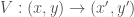
A Variation is a multivariable real number function with domain and codomain R^n. I will focus on the 2D version. Sometimes it can have a name map or a morphism, but I call it just a function. So our function converts a point $(x,y)$ into new point $(x',y')$ .

$V:(x,y)\rightarrow(x',y')$

Usually a Variation is designed as a whole class of functions, which means there are a few external parameters that you need to set to certain values in order to get a specific function. In such a case a different set of parameters will result in a different function.

The other parameter used is the ‘amount’ of the function. ‘amount’ is a special parameter which in almost all cases scales the resulting value.

So a more formal definition of our function is:

$V_{\alpha,P}=\alpha V_{P}(x,y)=(\alpha x',\alpha y')$ , where $\alpha \in [0,1]$ ; which means:

Variation V is a function with some sequence of parameters Ρ which is scaled by a factor α. Sequence of parameters Ρ is just a sequence of values which are used in definition of the function.

Although the domain is the whole R² space I usually only operate on [-3,3]x[-3,3] range.

Examples of Variations

Here are some basic ones (without parameters and with α=1):

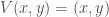
Identity –
- $V(0,0)=(0,0)$
- $V(1,1)=(1,1)$
Linear – $V(x,y)=(\alpha x,\alpha y)$
Sinusoidal –
- $V(0,0)=(0,0)$
- $V(1,-1)=(0,84,-0,84)$

Things get more complicated when we add sequence of parameters (and α=1). These definitions are function class definitions and by using specific parameters you will obtain unique functions.

PDJ – , where from .
- $V_{P}(1,-1) = (\sin{(-\pi)}-\cos{0}, \sin{2}-\cos{0}) = (-1,-0.09)$ , where $P = \{\pi,0,2,0\}$
Rectangles – , where from
- $V_{P}(1,-1) = (3\cdotp 1-1, -1\cdotp 1+1) = (2,0)$ , where $P = \{1,1\}$

How to draw it

Here is the template I use to draw. The general concept is to take every point from the [-3,3]x[-3,3] range, calculate the result of the function and draw it. This template draws a simple identity function:

void setup() {
  size(600, 600);
  background(250);
  smooth(8);
  noFill();
  stroke(20, 15);
  strokeWeight(0.9);

  x1=y1=-3;
  x2=y2=3;
  y=y1;
  step=(x2-x1)/(2.321*width);
}

float x1, y1, x2, y2; // function domain
float step; // step within domain
float y;

boolean go = true;
void draw() {
  if (go) {
    for (int i=0; (i<20)&go; i++) { // draw 20 lines at once
      for (float x=x1; x<=x2; x+=step) {
        drawVariation(x, y);
      }
      y+=step;
      if (y>y2) {
        go = false;
        println("done");
      }
    }
  }
}

void drawVariation(float x, float y) {
  float xx = map(x, x1, x2, 20, width-20);
  float yy = map(y, y1, y2, 20, height-20);
  point(xx, yy);
}

The result, which you can see here, is a grid that’s the result of rounding floating point values. By inserting the randomGaussian() function into the calculation I can distort the points a little and thus get a less rigid and more uniform look.

void drawVariation(float x, float y) {
  float xx = map(x+0.003*randomGaussian(), x1, x2, 20, width-20);
  float yy = map(y+0.003*randomGaussian(), y1, y2, 20, height-20);
  point(xx, yy);
}

Ok, now we are ready to plot our first functions!

Sinusoidal

Let’s start with a sinusoidal function.

V(x,y) = (αsin(x),αsin(y));

The code to draw this function looks like this:

void drawVariation(float x, float y) {
  PVector v = new PVector(x,y);
  float amount = 1.0;

  v = sinusoidal(v,amount);

  float xx = map(v.x+0.003*randomGaussian(), x1, x2, 20, width-20);
  float yy = map(v.y+0.003*randomGaussian(), y1, y2, 20, height-20);
  point(xx, yy);
}

PVector sinusoidal(PVector v, float amount) {
  return new PVector(amount * sin(v.x), amount * sin(v.y));
}

The top image is a plot with amount=1.0. The bottom image is an example where I used amount=3.0 to scale the resulting value up to the [-3,3]x[-3,3] range.

Hyperbolic

Another example is the hyperbolic function, which uses polar coordinates to calculate x and y.

PVector hyperbolic(PVector v, float amount) {
  float r = v.mag() + 1.0e-10;
  float theta = atan2(v.x, v.y);
  float x = amount * sin(theta) / r;
  float y = amount * cos(theta) * r;
  return new PVector(x, y);
}

PDJ

Now let’s draw functions from the PDJ class. The sequence of parameters are provided as external variables and used in the function.

// parametrization P={pdj_a,pdj_b,pdj_c,pdj_d}
float pdj_a = 0.1;
float pdj_b = 1.9;
float pdj_c = -0.8;
float pdj_d = -1.2;
PVector pdj(PVector v, float amount) {
  return new PVector( amount * (sin(pdj_a * v.y) - cos(pdj_b * v.x)),
                      amount * (sin(pdj_c * v.x) - cos(pdj_d * v.y)));
}

So, for example, when I set Ρ = {0.1, 1.9, -0.8, -1.2} I get:

But with Ρ={1.0111, -1.011, 2.08, 10.2} I get something very different:

See also Holger Lippmann’s works based on PDJ functions

Julia

The next function I want to show is Julia where random() function is used.

PVector julia(PVector v, float amount) {
  float r = amount * sqrt(v.mag());
  float theta = 0.5 * atan2(v.x, v.y) + (int)(2.0 * random(0, 1)) * PI;
  float x = r * cos(theta);
  float y = r * sin(theta);
  return new PVector(x, y);
}

Sech

And then there’s the last function, Sech, which is based on an hyperbolic functions:

float cosh(float x) { return 0.5 * (exp(x) + exp(-x));}
float sinh(float x) { return 0.5 * (exp(x) - exp(-x));}

PVector sech(PVector p, float weight) {
  float d = cos(2.0*p.y) + cosh(2.0*p.x);
  if (d != 0)
    d = weight * 2.0 / d;
  return new PVector(d * cos(p.y) * cosh(p.x), -d * sin(p.y) * sinh(p.x));
}

More to see

Click HERE to see the animations of 129 basic variations that I have created in Scratch

Now let’s complicate things!

Being aware now of the base functions (which are widely available: flame.pdf paper defines 48 of them, JWildfire code defines 200+ usable functions or classes of functions), we can then create new ones ourselves. Math theories (like group/ring theories, homomorphism, analysis, etc) with associativity and distributivity of operations give us recipes to build new functions from the others.

Let’s suppose we have variations $V(x,y)=(x',y')$ and $W(x,y)=(x'',y'')$ and we want to produce a new function Z. In order to do this we can then do any of the following:

Sum of the function: $(V+W)(x,y) = V(x,y)+W(x,y) = (x'+x'', y'+y'')$
Subtraction of the functions: $(V-W)(x,y) = V(x,y)-W(x,y) = (x'-x'', y'-y'')$
Combination of the function: $(V\circ W)(x,y) = V(W(x,y)) = V(x'',y'')$
Kind of differencial/derivative (it’s not strict differential): $\partial(V(x,y)) = \frac{V(x+h,y+h)-V(x,y)}{\sqrt{h}} = (\frac{x^*-x'}{\sqrt{h}}, \frac{y^*-y'}{\sqrt{h}})$ , where $V(x+h,y+h)=(x^*,y^*)$ and $h$ is some real number and $h\neq 0.0$
Multiplication: $(V*W)(x,y)=V(x,y)*W(x,y) = (x'*x'', y'*y'')$
Division: $(\frac{V}{W})(x,y)=\frac{V(x,y)}{W(x,y)} = (\frac{x'}{x''},\frac{y'}{y''})$ , where when denominator is 0, value is also 0 (just to simplify things)
Power: $V^{n}(x,y) = V^{n-1}(x',y')$ or as recursive combinations: $V(V(V(V(\cdots V(x,y)\cdots ))))$

You can of course mix all of the above to create a bunch of new and unique functions. For example, you can create function which is a sum of combination of power of division of few base functions. Or whatever else you want.

The sum, subtraction, multiplication and division of functions can be coded like this:

PVector addF(PVector v1, PVector v2) { return new PVector(v1.x+v2.x, v1.y+v2.y); }
PVector subF(PVector v1, PVector v2) { return new PVector(v1.x-v2.x, v1.y-v2.y); }
PVector mulF(PVector v1, PVector v2) { return new PVector(v1.x*v2.x, v1.y*v2.y); }
PVector divF(PVector v1, PVector v2) { return new PVector(v2.x==0?0:v1.x/v2.x, v2.y==0?0:v1.y/v2.y); }

Combination can be obtained like this (julia o sech)

  v = julia(sech(v,amount),amount);

Power, which is multiple combination of the same function, can be coded like this (hyperbolic^5 = hyperbolic(hyperbolic(hyperbolic(hyperbolic(hyperbolic)))) )

  for(int i=0;i<5;i++) v = hyperbolic(v,amount);

And an example of a differential of pdj function:

PVector d_pdj(PVector v, float amount) {
  float h = 0.1; // step
  float sqrth = sqrt(h);
  PVector v1 = pdj(v, amount);
  PVector v2 = pdj(new PVector(v.x+h, v.y+h), amount);
  return new PVector( (v2.x-v1.x)/sqrth, (v2.y-v1.y)/sqrth );
}

hyperbolic + pdj

  v = addF( hyperbolic(v,amount), pdj(v,amount) );

julia – hyperbolic

  v = subF( julia(v,amount), hyperbolic(v,amount) );

sech * pdj

  v = mulF( sech(v,amount), pdj(v,amount) );

hyperbolic / sech

  v = divF( hyperbolic(v,amount), sech(v,amount) );

d(pdj)

  float amount = 3.0; // scale up
  v = d_pdj(v,amount);

julia o hyperbolic = julia(hyperbolic)

  v = julia(hyperbolic(v,amount),amount);

hyperbolic ^ 10

  for(int i=0;i<10;i++) v = hyperbolic(v,amount);

[julia((hyperbolic + julia o sech) * pdj) – d(pdj)]^3

  for(int i=0;i<3;i++)
    v = subF(julia( mulF(addF(hyperbolic(v,0.5),julia(sech(v,1),0.5)),pdj(v,1)),2.5),d_pdj(v,1));

Folding

In the above examples you can see that some of the points have escaped outside of the screen. The main reason is that the values exceeded -3 or 3. To keep them inside our area we have to force them to be in the required range of values. There are a couple of strategies for achieving this. I will describe two of them: modulo and sinusoidal.

I will use pdj + hyperbolic * sech function with amount = 2

  float amount = 2.0;
  v = addF(pdj(v,amount),mulF(hyperbolic(v,amount),sech(v,amount)));

Modulo

The first strategy is to treat the screen as a torus (points that exceed the screen area will reappar on the opposite side: top <> down, left <> right). The formula for this wrapping is documented below. It is called after the function has been calculated.

  v.x = (v.x - x1) % (x2-x1);
  if(v.x<0) v.x += (x2-x1);
  v.y = (v.y - y1) % (y2-y1);
  if(v.y<0) v.y += (y2-y1);
  v.x += x1;
  v.y += y1;

Sinusoidal

The second strategy is to wrap the points using a sinus function, which moves between -1 to 1. With amount=3 you get the required range.

  v = sinusoidal(v,(x2-x1)/2);

Towards fixed point

In maths a ‘fixed point’ is a special point a where f(a) = a. If the function has a special characteristic (is a contraction mapping) a fixed point can be calculated by using the power of the function as defined above. Just call f(f(f(f(f(f….))))). In our case we operate on a set of points (range [-3,3]x[-3,3]) and our “fixed point” can also be set (if exists). So let’s try to modify our code a little and draw each step for a certain power of our function.

Let’s create a function v = sinusoidal o julia o sech calculate v(v(v(v(…)))) and draw each step: first v, then v(v), v(v(v)), in order to finish at some chosen number.

Our algorithm will look like this:

set n = 3
choose a point p = (x,y)
calculate new point p = sinusoidal(julia(sech(p)))
draw point p
repeat n (=3) times steps 3-4 (using newly calculated point p)
go to 2

But first we need to adjust the step value and set the stroke color to be slightly lighter

  stroke(60, 15);
  //...
  // more points drawn in drawVariation, bigger step
  step=sqrt(n)*(x2-x1)/(2.321*width);

And adapt drawVariation()

int n=1;
void drawVariation(float x, float y) {
  PVector v = new PVector(x, y);

  for (int i=0; i<n; i++) {
    v = julia(sech(v, 1), 1);
    v = sinusoidal(v, (x2-x1)/2);
    float xx = map(v.x+0.003*randomGaussian(), x1, x2, 20, width-20);
    float yy = map(v.y+0.003*randomGaussian(), y1, y2, 20, height-20);
    point(xx, yy);
  }
}

The following images represent represent values of n = 1, 2, 4, 8, 16, 32, 64, 128.

For high n the sequence will finally result in this (it’s a fixed point of our function)

Folds2d

To produce my works I prepared a few more things to have more variety of functions and semi-artistic look. These are:

JWildfire wrapper for Processing (to get all Variations included there)
Random formula generator with evaluation
Randomization of parameters
Noisy, gray canvas
High resolution rendering
Fixed point option
Scaling / translating range
Various folding options
and probably few more

Final notes

I would like to THANK Jerome Herr for review of this article. Thank you very much man!

Don’t forget to visit his page: http://p5art.tumblr.com/

Questions/Errors? generateme.blog@gmail.com

6 Comments to “Folds”

Keith Peters says:

April 14, 2016 at 1:06 pm

Very nice. I started porting some of this to js/canvas. http://jsbin.com/kuneye/edit?js,output

LikeLiked by 1 person

- tsulej says:
  
  April 14, 2016 at 1:24 pm
  
  Cool! Thnx! My advice is to use gaussian random to distort points rather than uniform distribution.
  
  LikeLike
  
  - Keith Peters says:
    
    April 14, 2016 at 2:07 pm
    
    yeah, unfortunately, I’d have to write my own or find one somewhere. Cool stuff, fractal flames has been on my list of things to get into for years.
    
    LikeLiked by 1 person
  - tsulej says:
    
    April 14, 2016 at 2:37 pm
    
    Use this snippet (taken from processing2):
```
float nextGaussian = 0;
boolean haveNextGaussian = false; 
float randomGaussian() {
  if(haveNextGaussian) {
    haveNextGaussian = false;
    return nextGaussian;
  } else {
    float v1,v2,s;
    do {
      v1 = 2 * random() - 1;
      v2 = 2 * random() - 1;
      s = v1 * v1 + v2 * v2;
    } while (s >=1 || s == 0);
      
    float mult = sqrt(-2 * log(s) / s);
    nextGaussian = v2 * mult;
    haveNextGaussian = true;
    return v1 * mult;
  }
}
```
    LikeLike
Taxicletter says:

April 21, 2016 at 6:52 pm

Just looking at the pictures: Lovely! Nice on my eyes. Later, I will try to understand the theory behind it. I’m a very beginning Processing-enthousiast with too little time 🙂

LikeLiked by 1 person

Generating animated gifs from random 2D transformations – necessary-disorder tutorials says:

January 30, 2018 at 1:11 pm

[…] Here is a tutorial that presents some 2D transformations and explains how to render them nicely with Processing : https://generateme.wordpress.com/2016/04/11/folds/ […]

LikeLike

GenerateMe

Folds

by tsulej

folds2d.tumblr.com

Variations

Examples of Variations

How to draw it

Sinusoidal

Hyperbolic

PDJ

Julia

Sech

More to see

Now let’s complicate things!

hyperbolic + pdj

julia – hyperbolic

sech * pdj

hyperbolic / sech

d(pdj)

julia o hyperbolic = julia(hyperbolic)

hyperbolic ^ 10

[julia((hyperbolic + julia o sech) * pdj) – d(pdj)]^3

Folding

Modulo

Sinusoidal

Towards fixed point

Folds2d

Final notes

6 Comments to “Folds”

Leave a comment Cancel reply

GenerateMe

Folds

by tsulej

folds2d.tumblr.com

Variations

Examples of Variations

How to draw it

Sinusoidal

Hyperbolic

PDJ

Julia

Sech

More to see

Now let’s complicate things!

hyperbolic + pdj

julia – hyperbolic

sech * pdj

hyperbolic / sech

d(pdj)

julia o hyperbolic = julia(hyperbolic)

hyperbolic ^ 10

[julia((hyperbolic + julia o sech) * pdj) – d(pdj)]^3

Folding

Modulo

Sinusoidal

Towards fixed point

Folds2d

Final notes

Share this:

Related

6 Comments to “Folds”

Leave a comment Cancel reply